Custom spatial filters

User Guide:

Buffer overscan region Customizing the edge extraction settings

Reference:

MbufAlloc1d MbufAlloc2d MbufControlNeighborhood MbufPut MbufPut2d MimConvolve

Not available in MIL-Lite

Available in MIL

Spatial filtering operations include operations such as smoothing, denoising, edge enhancement, and edge detection.

Spatial filtering operations compute results based on an underlying neighborhood process: the weighted sum of a pixel value and its neighbors' values. There are two types of spatial filters: Finite Impulse Response (FIR) filters and Infinite Impulse Response (IIR) filters. FIR filters operate on a finite neighborhood, while IIR filters take into account all values in an image. In MIL, you can specify either a predefined or a custom FIR or IIR spatial filter.

Finite Impulse Response (FIR) filters

For FIR filters, the weights are known as the kernel values. These kernel values determine the operation type of the spatial filter. For example, applying the following FIR filter results in a sharpening of the image:

Whereas, applying the following FIR filter smooths an image (it also increases the intensity of the image by a factor of 16, so you will need to normalize the convolution result):

When using FIR filters, the dimensions of the kernel determine the size of the neighborhood that is used in the operation. The result of the operation is stored in the destination buffer at the location corresponding to the kernel's center pixel. When the kernel has an even number of rows and/or columns, the center pixel is considered to be the top-left pixel of the central elements in the neighborhood.

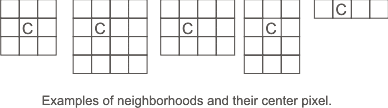
Calculate the X-coordinate of the top-left pixel of the central elements, as follows:

If the width (SizeX) of the kernel is an odd number, the X-coordinate is (SizeX-1)/2.
If the width (SizeX) of the kernel is an even number, the X-coordinate is (SizeX/2)-1.

To calculate the Y-coordinate of the top-left pixel of the central elements, the same rules apply.

Regardless of the location of the center pixel, there will be some border pixels that have an incomplete neighborhood. To deal with this issue, the image buffer is overscanned. There are several types of overscan. A transparent overscan uses the parent buffer to provide the overscan pixels needed for the border calculation. If the parent buffer is not available, a mirror overscan is performed. A mirror overscan specifies that the overscan pixels will be a mirror copy of the source buffer's border pixels. A replacement overscan allows you to specify a specific value for the overscan pixel values during processing. For more information on overscan, see the Buffer overscan region section of Chapter 19: Data buffers.

If the predefined FIR filters provided by MimConvolve() do not meet your requirements, you can create your own custom FIR filter. To define your own custom FIR filter:

Allocate a kernel buffer, using MbufAlloc1d() or MbufAlloc2d() with M_KERNEL. The kernel size is specified when allocating the kernel buffer. Note that the kernel size can be constrained by the available resources.
Load the required kernel values into this kernel buffer, using MbufPut() or MbufPut2d().
If required, modify the setting of the operation control types associated with your custom filter, using MbufControlNeighborhood(). The operation control types determine how the convolution operation will be handled. You can control:
- Whether or not the absolute value of the result is taken (M_ABSOLUTE_VALUE).
- The division (normalization) factor to apply to the result (M_NORMALIZATION_FACTOR).
- Whether or not to saturate the result (M_SATURATION).
- The position of the center pixel (M_OFFSET_CENTER_X and M_OFFSET_CENTER_Y).
- How the operation handles the borders (overscan) of the source buffer (M_OVERSCAN and M_OVERSCAN_REPLACE_VALUE). If overscan is disabled, the border pixels of the source image are not processed if additional processing time is needed.

To apply your own custom FIR filter, call the MimConvolve() function, specifying the identifier of the required kernel buffer (KernelBufId).

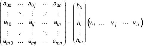
To increase the speed of the convolution operation when using your custom FIR filter, MimConvolve() will automatically separate large kernels, if separable, into two 1-dimensional kernels (a_ij = h_iv_j ). Performing two separate convolutions, once with H_nx1 and once with V_1xm can be faster and is equivalent to performing one convolution operation using the original A_mxn kernel. MIL will internally separate large kernels when it detects that the separation results in better performance. The following displays an A_mxn kernel separated into two 1-dimensional kernels (H_m and V_n ).

Infinite Impulse Response (IIR) filters

When using IIR filters, the weights are automatically determined by the type of filter, the mode of the filter, the type of operation to perform, and the degree of smoothness (strength of denoising) applied by the filter.

The type of filter determines the distribution of the neighborhoods' influence. MIL supports two types of IIR spatial filters: Canny-Deriche filter and Shen-Castan filter. For the Canny-Deriche filter, the neighborhoods' influence decreases much slower as the distance from the central pixel increases, compared to the Shen-Castan filter. For more information, see the Customizing the edge extraction settings section of Chapter 8: Edge Finder.

There are two modes in which to perform the filter: kernel mode and recursive mode. When performing an IIR filter in recursive mode, the kernel size would be theoretically infinite if this mode actually used a kernel. When performing a custom IIR filter in kernel mode, the filtering is done using a kernel approximation (FIR) of the filter. Kernel mode is not available for a predefined IIR filter. Kernel mode has been provided to take advantage of your system if it is optimized for kernel mode; kernel mode is typically not as efficient as recursive mode unless your system is optimized for kernel mode.

If the predefined IIR filters provided by MimConvolve() do not meet your requirements, you can create your own IIR filter. To define your own IIR filter:

Allocate a kernel buffer, using MbufAlloc1d() or MbufAlloc2d() with M_KERNEL.
Use MbufControlNeighborhood() and specify appropriate M_FILTER_TYPE, M_FILTER_MODE, M_FILTER_OPERATION, and M_FILTER_SMOOTHNESS operation control type settings.

Note that the kernel size specified during allocation is ignored, unless you will be performing the filter in kernel mode; in which case, the specified kernel size can be constrained by the available resources. In addition, regardless of the filter mode, when using IIR filters the kernel values specified in the kernel buffer are ignored; they are determined automatically.
If required, modify the setting of your custom filter, using MbufControlNeighborhood(). The operation control types determine how the convolution operation will be handled. You can control:
- Whether or not the absolute value of the result is taken (M_ABSOLUTE_VALUE).
- The division (normalization) factor to apply to the result (M_NORMALIZATION_FACTOR).
- Whether or not to saturate the result (M_SATURATION).

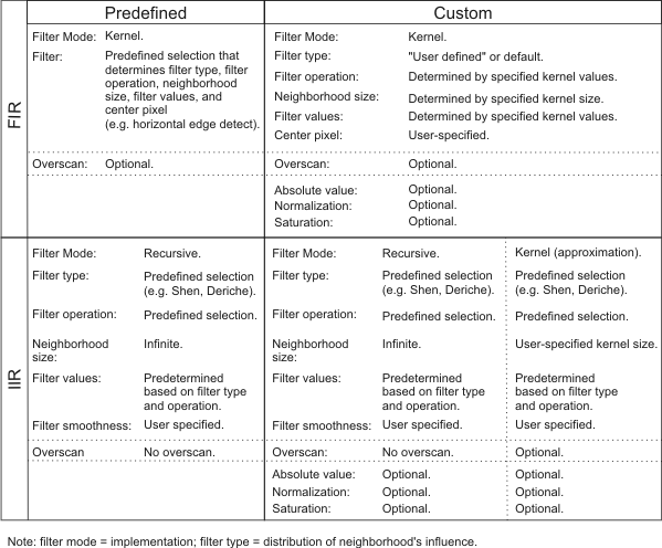
A summary

The following is a summary of spatial filtering options.

An example

The following is an example of a spatial filtering operation using a custom FIR filter with a 3 by 3 kernel.

mimconvolve.cpp