Advanced techniques
- See also

 Availability
 Previous
- Next

-
If the classification is based on a small area (for example, a small scratch), relative to the size of the entire scene, and you cannot otherwise delimit the area (for example, with fixturing). In such cases, using a local view of the data can improve the classification's robustness.
-
If the approximate locations of the classes (for example, the defects) are important for the application.
-
M_TARGET_IMAGE_SIZE_X = M_SIZE_X + m * M_STEP_X , where m is an integer that is greater than or equal to 0.
-
M_TARGET_IMAGE_SIZE_Y = M_SIZE_Y + n * M_STEP_Y , where n is an integer that is greater than or equal to 0.
-
Decide the size of the training images. This is the size of your tile (receptive field).
-
Extract the tile like regions from your source images and save them as their own image. The extraction can be random or intelligent.
Random extraction typically involves generating a certain number of tile like images from arbitrary locations in every source image. The number of tiles to extract from every source image depends on your accuracy requirements and the receptive field (tile size).
Intelligent extraction typically involves generating the tile like images based on what you want to classify (such as the defect) in the source images. To do this, you can:
-
For each image, brush over the pixels that represent what you want to classify (segment). Simple graphics editors typically provide this functionality. Conventionally, the brushing color should represent the class label. For example, if your DefectPit class is Class1 and your DefectScratch class is Class2, you should identify them using a color value of 1 and 2. Once you have brushed the pixels, you can save a version of these images where every brushed pixel value is maintained, and every other pixel value, which will represent the background, is set to a consistent color. Conventionally, background pixels are set to 0 (black) and the Background class has the label 0.

-
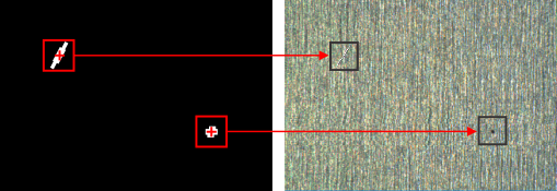
Pass the brushed version of these images to the Blob analysis module and locate the blobs (which are, in fact, the defects).

You now know where and what the defects are, and you can correlate this information to extract the corresponding tiles that enclose those defects from the original source images that you collected. Note, having a background of 0, as previously suggested, makes these images easier to use with the Blob Analysis module.
-
Extract the tiles used to train the Background class. For each source image, you can either randomly extract tiles (many of which will contain the background) or you can systematically extract all possible tiles.

-
-
Label every extracted tile as the class they represent (the ground truth), including the background class. This process is simplified if you performed an intelligent extraction.
Once the tile images are the correct size and labeled, add them to your datasets and proceed with typical training techniques.
-
Transformation-related.
Examples include translation, rotation, flip, shearing, aspect ratio, and scale.
-
Intensity-related.
Examples include smoothing, adding noise, brightness variations.
-
Only allow augmented entries in the training dataset. In this case, augmented entries also refers to the entries used to augment them. All of these entries must only be in the training dataset.
-
Augment your data after splitting it into different datasets. It is not recommended to call MclassSplitDataset() to create the development dataset or testing dataset if your source dataset contains augmented entries.
Identify augmented entries by calling MclassControlEntry() with M_AUGMENTATION_SOURCE.
-
Disregard bagging information if your training dataset has augmented entries.
-
Keep the source entry and its augmented entries in one dataset. The source and its variations are considered part of the augmentation.
-
Plan for mechanisms to efficiently collect more data from a deployed system.
-
Archive the datasets to potentially further improve a network and assess the performance improvement.
-
Images are acquired by batches of product of the same type / aspect.
-
Images are acquired by batches at different periods of the day, under distinct illumination conditions.
-
Only a ROI within an image needs to be classified and the location of this ROI can be established using other means such as from a pattern matching occurrence.
-
Multiple ROIs within an image with different labels need to be extracted, either manually or automatically using a segmentation technique, for example.
-
Fixturing, if applicable, might be used to also correct an image or a ROI of geometric variations (rotation, scale, or translation). The reduction of possible variations simplifies the classification problem, increasing the chance to obtain a better/faster trained network.
-
Systematic data preparation errors.
-
A significant amount of mislabeled data that you must fix.
-
An inappropriate data augmentation strategy (for the training dataset) that does not reflect the original goal.
This section describes advanced techniques, generally related to your datasets and training.
Coarse segmentation
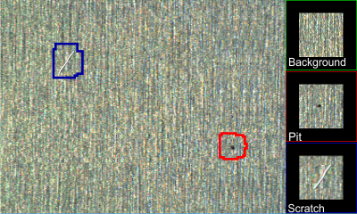
Typical image classification applications predict the class to which an entire image belongs. When using a coarse segmentation approach, MclassPredict() determines the class to which smaller regions (tiles) in an image belong. This is typically done when you want to detect defects, such as pits or scratches on highly textured metal surfaces.
When using this approach, you often know what the target (prediction) image is; for example, you know that you are looking at images of metal. What you don't know, and want you want to find out, is whether that image has what you are interested in classifying, such as defects.
The main reasons to use a coarse segmentation approach are:
Performing coarse segmentation
The classification (training) process for coarse segmentation is the same as any typical image classification process, except your training images are smaller (typically, significantly smaller) than your target images (prediction) and represent tile like areas that enclose what you want to classify, including defects and the background.

Although training images are smaller, you must have many of them in your datasets, they must properly and proportionally represent all the different classes (including the background), must all be the same size, and must adhere to the receptive field (image size) requirements of the predefined CNN that you are using (just like a typical image classification process). For more information about the receptive field requirements of the predefined CNNs, see the Predefined CNN classifiers to train subsection of the Training: CNN section earlier in this chapter.
When using a coarse segmentation approach, the sizes of the target images (MclassPredict()) can vary; however, they must always be larger than the training images (and also the CNN's source layer), in both the X- and Y-dimension. If the dimensions of the target images and the training image (source layer) are the same, then you are performing typical image classification.
To specify target images that are larger than training images, you must call MclassControl() with M_TARGET_IMAGE_SIZE_X and M_TARGET_IMAGE_SIZE_Y. These dimensions must be greater than the CNN's source layer, which you can inquire with M_SIZE_X and M_SIZE_Y.
The increment by which you can increase the dimensions of the target image depends on the size of the classifier's source layer and step. The following calculations indicate how to establish these dimensions:
Note, coarse segmentation is not a fundamentally different type of image classification. There is no setting to specify that you are performing coarse segmentation. Coarse segmentation is the implied approach when your receptive field (the dimensions of the training images, which corresponds to the dimensions of the source layer) is smaller than the target image with which to predict.
Training images
Ideally, you should be able to easily collect and label the data with which to train. However, collected data usually consists of images that correspond to target images used at prediction, and not to smaller regions (tiles).
You must therefore extract those tiles (regions of interest) from your data (images) and use them as your training images. You can do this any way you see fit, as long as you end up with the proper set of labeled images in your datasets. The following steps provide a basic methodology for establishing the tile like training images from larger images:
Coarse segmentation results (classification map)
With typical image classification applications, results are returned for the entire target image, such as the class score (for example, the score for Class0 and Class1). When using a coarse segmentation approach, those results are returned for every tile that is established in the image. These results can be seen as a type of map result.
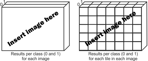
The number of prediction results (the size of the classification map) returned for every target image depends on the size of the tiles (which are used to train the context), the size of the target image, and the step size of the predefined CNN. The size of the tiles must also adhere to the predefined CNN's receptive field requirements.
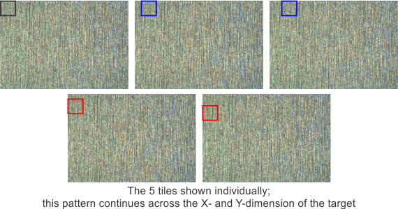
The following example shows a target image and one tile for which results are returned.

If you specify a medium predefined CNN, which has a minimum image size of 83 pixels and a step size of 8 pixels, results are actually returned for that one tile (for example, 83 x 83) and for all tiles like it that are 8 pixels to the right and to the bottom of it. The following example shows an approximation of 5 such tiles. As you can see, the borders of every tile overlap, given that the step is smaller than the tile's dimensions.

Although borders can overlap, each tile is its own region and all tiles are the same size. The following example shows how each of the 5 tiles would look on the target, if the other tiles are hidden.
As previously discussed, when using a coarse segmentation approach, a map of results is returned, corresponding to every tile. Since areas (pixels) in the target can overlap across multiple tiles, given the step and tile (receptive field) size, it can be difficult to decipher the correspondence between each map result and its tile in the target image. The following example approximates how tiles in the target image, and in the corresponding map result, might look.
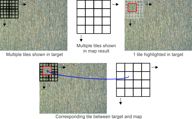
To correlate the map results to their corresponding tiles (receptive field) in the image, call MclassGetResult() with M_CLASSIFICATION_MAP_OFFSET_..., M_CLASSIFICATION_MAP_SCALE_..., and M_CLASSIFICATION_MAP_SIZE_....
To retrieve the dimensions of the tile (the receptive field), use M_RECEPTIVE_FIELD_SIZE_.... To retrieve the number of resulting tiles, use M_CLASSIFICATION_MAP_SIZE_.... Since results are returned for every class per tile, the total number of results returned for an image is: M_CLASSIFICATION_MAP_SIZE_X x M_CLASSIFICATION_MAP_SIZE_Y x M_NUMBER_OF_CLASSES.
Note, for typical image classification, you can consider the size of the tile as equivalent to the size of the target image (therefore, 1 tile/result per class for each image).
Drawing coarse segmentation results
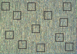
Prediction results from a coarse segmentation can prove complex to decipher, given that you can have multiple results for each training image. For example, a coarse segmentation prediction can identify two classes in the following target image.

By calling MclassDraw(), you can draw a contour around the classes found, as well as the corresponding color of every class, including the background. Such drawings help you better understand the results of the prediction.
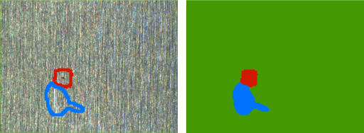
Note, to perform these drawing operations, specify M_DRAW_BEST_INDEX_CONTOUR_IMAGE (for the image on the left) and M_DRAW_BEST_INDEX_IMAGE + M_PSEUDO_COLOR + M_REPLICATE_BORDER (for the image on the right).
Augmentation
Data augmentation is a technique to synthetically generate more samples (entries) from a limited dataset to be used during training. Therefore, if you do not have enough training data, you can use augmentation to synthesize more. The ultimate goal is to have training data that is a full representation of all expected variations and conditions. If you cannot get the actual data, augmentation can be a solution.
Data augmentation can prevent overfitting and can improve accuracy as well as robustness. Various types of data augmentation are available, such as:
To specify these operations, and others, you must call MimControl() with an augmentation context, allocated using MimAlloc(). To run the actual augmentation, call MimAugment().
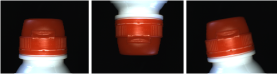
The application of a specific augmentation type depends on the problem definition. The augmentation should make sense in the context of the application. For instance, if the rotation of an object does not happen in the real application or it changes the label of the image, then rotation should not be applied as an augmentation (or, only a few degrees of rotation could be used, if necessary).
The following bottle cap inspection example illustrates the point. In this case, the original image is shown first, then, a rotation of 180 degrees is shown, but this actually can never happen in the application, so it must not be included in the set of augmented images that you use. Finally, the third image shows an 10 degree rotation, which can happen (the bottle might shake and tilt on the conveyor), so this augmentation can be used.
Other types of data augmentations might be needed in addition to just supplementing original variations. For example, over time, images might be subject to change of focus and noise. These changes could have a noticeable impact on the network's accuracy. Hence, to overcome this problem, these artifacts should also be simulated through data augmentation.
In some cases, the original dataset is not balanced. This means that there is a significant difference in quantity of labeled data between the different classes. As a result, the network might give too much importance to the class with more data. One solution to an imbalanced dataset is data augmentation.
For example, 1000 images are available for class A (non-defective parts) and only 50 images are available for class B (defective parts). In this situation, more data augmentation could be applied for class B to narrow the gap between the two classes.
Such augmentations, to a single class, require especially prudent considerations, since you do not want the classifier to unrealistically learn how to identify that class (the augmentations must always reflect the overall problem). This in part explains why, as previously mentioned, you must not add augmented data to the development dataset or the testing dataset, since they are use to regulate and help you identify misguided classifications.
For more information about setting up, performing, and analyzing an augmentation for images, see the Augmentation section of Chapter 5: Specialized image processing.
A features dataset can also be augmented. For example, if one of the features (numerical values) in a dataset entry refers to the width of a blob, you can add entries that are a certain percentage bigger or smaller. Those additional entries should be considered augmented. Also, entries in a features dataset could have been added from a blob analysis that you performed on images. If some of those images were augmented, then the corresponding features should be considered augmented also.
Note the following recommendations:
Note, original images should be a little larger than those in the final application, to ensure that augmented images do not contain overscan pixels. In the final training dataset, you can crop the images to meet the application's size requirements.
Advanced analysis of your training
An advanced analysis of your training refers to a more in-depth and granular investigation into what was properly and improperly classified. Such techniques can shed light on why your training is proving unsuccessful and how to fix it.
Confusion matrix
The confusion matrix is a type of table, in a matrix format, that presents information about how many entries were correctly and incorrectly classified during training. A correctly classified entry means that its predicted class is the same as the ground truth for that class (the expected class).
For example, the following confusion matrix was calculated after the training was done using a development dataset with 3 classes (A, B, and C) and 500 entries (images) representing each one.
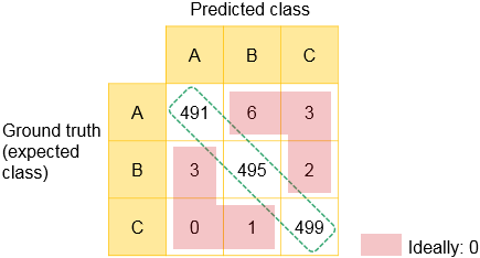
The cells where the classes in the ground truth row on the left intersect with the corresponding classes in the predicted column at the top indicate the number of development dataset entries that were properly classified as that class. If the classifier is perfect, the number of predicted classes would always equal the number of ground truth (expected) classes; this would result in a value of 0 in every other cell. In this example, the perfect result would be to have 500 in every intersecting cell.

By examining the values in the intersecting cells, and in the other cells, you can understand the proportions between the true positives, the false positives, the true negatives, and the false negatives. Theoretically, the confusion matrix allows you to retrieve performance metrics, such as the classifier's precision, accuracy, recall (also known as sensitivity), and F1 precision. In particular, the recall metric is an important indicator of the performance of the classifier, especially when in the presence of unbalanced datasets.
Although counter intuitive, it can be preferable for certain applications to actually have some false classifications. Generally, if a classification is incorrect, it is either a false positive or false negative. The classifier is either wrong about what it thought was right (false positive classification) or it is wrong about what it thought was wrong (false negative classification). This information can prove invaluable, not only to help you adjust your training, but also to develop a better classifier for your specific application. For example, you might want to err on the side of false positives for a defective class, or you might want to err on the side of false negatives for a good class to maintain yields and reduce waste.
The confusion matrix is available as both a CNN and tree ensemble training result, by calling MclassGetResult() with the related setting, such as, M_TRAIN_DATASET_CONFUSION_MATRIX, M_DEV_DATASET_CONFUSION_MATRIX, or M_OUT_OF_BAG_CONFUSION_MATRIX (for tree ensemble).
Score distribution
The classifier returns a score for each class. The image that you are classifying is, as expected, associated with the class with the highest score. The highest score is always greater than 100/N , where N is the number of classes.
It is possible that false positives are more important than false negatives, and vice versa. Other than using the score to identify the best class, you can use it to take further decisions about the classified image. For example, a weak highest score, such as 51% in a binary classification problem, can result in rejecting the part to minimize the false positive rate.
Analyzing the distributions of the scores, per expected class, can facilitate setting up a threshold decision to establish what is the lowest acceptable highest score before the classification result is rejected. An example of this is shown in the following image.
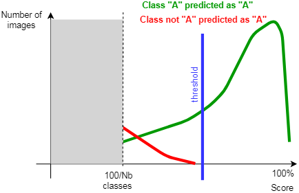
You can construct score distribution information like this using results that you can retrieve by calling MclassGetResult().
Improving a deployed network
It might be difficult to collect enough data to fully cover all variations of the final application. The development dataset accuracy might be overestimating the real performance of the application. In such cases, the deployed system can also collect additional data of interest to add to the training dataset. The increased dataset can be further used to improve the network through fine-tuning.
A threshold on the score can be used to select the images to collect, typically the ones classified with a low confidence. These images will need to be manually verified and labeled later by an expert and added to the existing training and development datasets. If, after fine-tuning, the performance of the network is improved, the new network can be re-deployed in the field.
To improve your classifier's training, it is recommended to:
Shuffling
It is likely that the data gathering process leads to correlated sequences of images as, often times, the training images are captured sequentially. For example:
The presence of these sequences can compromise the training process with the risk of reducing the training speed and quality. A uniform distribution of the data is important to better generalize and remove unwanted biases from the training process. To remove the potential presence of sequences, the order of the training data is shuffled, ideally per class.
Extracting
In some applications, there might be a need to extract and to preprocess a region of an image to be classified. For example:
Note that some or all steps involved in the extraction of the data might also have to be applied before the inference (prediction) in the final application.
Preprocessing
Ideally, you can feed your captured images directly to the network. However, images can require preprocessing first.
You must not preprocess data if you intend to augment it (you can preprocess it afterward). Images should have the same number of channels, size, and bit depth.
Oftentimes, images need to be down-sampled before being fed to a network. Big images slow down training and prediction (inference) speed. They also require more memory for training. In other cases, like the MIL seafood example (ClassSeaFoodInspect.cpp), smaller objects are extracted from larger images. This can be done by simply applying a child buffer whose location and dimensions are established from other operations like blob analysis. Care must be taken to ensure that the preprocessing step does not produce adverse effects. For example, down-sampling should not eliminate important features in the image.
Preprocessing can also improve the classification accuracy, especially when the training dataset is small, by removing the uninformative parts of the image, such as borders. This allows the classifier to learn the user intended features faster. You should apply the same preprocessing to the images used for training and for prediction.
Pitfalls
Adjusting made for bias and variance analysis can prove insufficient for improving your classifier's training. This can be a sign that hidden or unsuspected issues might exist, which often has to do with your data.
Data quality
Carefully review your datasets and look for:
Data distribution
Typically, the data in all your datasets come from the same distribution (the same environment and setup). However this is not always the case.
For example, the training dataset might contain images from different sources or systems, such as images of fabrics from the internet and also from the target application, while the development dataset might only contain images of fabrics taken from the target application. In such cases, you can create another dataset (the training development set) which has images from the same distribution as the training dataset, and use it to determine the presence of data mismatch issues between the training dataset and the development dataset.
Unbalanced data
As previously discussed, you should collect and label as much data as possible for all classes. However for some applications this can be impossible, and you might have highly unbalanced data; for example, a dataset might contain 1000 images representing ClassA (these can be the valid versions of the image), but only 25 bad images representing ClassB (these can be the invalid versions of the image).
With such an imbalance, the global accuracy can lead to a misleading interpretation of the classifier's true performance. You should therefore verify the accuracy per class (this is also known as recall). Consider a dataset that has 99% of its content represented by ClassA and 1% of its content represented by ClassB; this dataset's global accuracy can be as high as 99%, even though the classifier fails 100% of the time when trying to classify ClassB.