Distance between colors
- See also

 Availability
 Previous
- Next

-
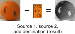
When the sources are images, McolDistance() calculates a point-to-point distance, while McolMatch() uses color statistics (average color). McolMatch() calculates the distance between each color-sample's statistic and each target area's statistic, or between each color-sample's statistic and each pixel in each target area, depending on the operation mode specified with McolSetMethod().
-
McolDistance() results are from two specified sources. However, McolMatch() results can come from several color-samples, or even from background and outlying regions.
-
If you are only interested in distance values, McolDistance() can be more convenient to use than McolMatch(), since McolDistance() requires less setup, does not perform a matching operation, and results are returned directly to the function.
-
Unlike McolDistance(), McolMatch() takes the specified context's color space into account; it also offers more options than McolDistance(), such as converting to the CIELAB color space and operating on specific color bands.
-
Euclidean (M_EUCLIDEAN).
-
Mahalanobis (M_MAHALANOBIS).
-
Manhattan (M_MANHATTAN).
-
Delta-E (M_DELTA_E).
-
Advanced distance types, as established by the standards of the International Commission on Illumination (CIE).
These distance types are only available for color matching (McolMatch()).
-
r1 and r2 represent the first color component of the first and second source color.
-
g1 and g2 represent the second color component of the first and second source color.
-
b1 and b2 represent the third color component of the first and second source color.
-
r1 and r2 represent the first color component of the first and second source color.
-
g1 and g2 represent the second color component of the first and second source color.
-
b1 and b2 represent the third color component of the first and second source color.
-
x represents the first source color.
-
u represents the average of the second source color.
-
sigma is for the covariance matrix of the second source color.
-
CMC (M_CMC_ACCEPTABILITY and M_CMC_PERCEPTIBILITY).
These distance types are generally intended for the textile industry and allow for lightness and chroma factors based on either acceptability or perceptibility requirements.
-
CIE94 (M_CIE94_GRAPHIC_ARTS and M_CIE94_TEXTILE).
These distance types are similar to CMC but allow for weighting factors based on color tolerances for either the graphic arts industry or the textile industry.
-
CIEDE2000 (M_CIEDE2000).
This distance type is similar to CIE94, but is generally more robust regarding the effect of lightness on color. If M_DELTA_E is proving ineffective, you might want to try M_CIEDE2000 as a first alternative.
-
The first principal component, indicated by the red lines. Each first principal component represents the direction of greatest standard deviation for its group of pixels.
-
The mean color, indicated by the intersection of the blue line with the first principal component.
It might be useful to calculate the distance between colors, for example, to find flaws in an image by comparing it to a perfect version of the image (golden template), or to a color constant.
Distances between colors can either be calculated using McolDistance(), or when matching colors with McolMatch(). If required, you can normalize distance results. For more information, see the Distance normalization settings subsection of the Advanced color matching settings and concepts section later in this chapter.
Using McolDistance(), you can calculate the point-to-point distance between colors in two sources. The first source must be an image, while the second source can be: an image, a color constant, a covariance matrix, or the covariance of a specified image. Results are written to the destination image.
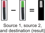
To ignore unwanted pixels in the distance calculation, you can use McolDistance() with a mask image, within which you must identify the masked (non-zero) pixels. Set unmasked pixels to 0 in the mask. The color distance is calculated only for the masked (non-zero) pixels within the intersection of the source, destination, and mask images, with the assumption of a common origin at the top-left corner.
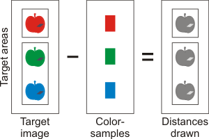
Color distances are also calculated when determining which color-sample best matches an image area. Therefore, you can retrieve distance results, after calling McolMatch(). The following image shows how distances between the target areas and multiple color-samples can be drawn. The distances drawn correspond to the distances between the target areas and their best-matched color-samples. Note that this is unlike McolDistance(), which can only calculate the distance between 2 sources.
For more information on retrieving color distances when matching colors, see the Image results subsection of the Color matching section later in this chapter.
When calculating the color distance, make sure the color data that you provide is compatible. For example, you will not receive an error if you try to calculate the distance between an RGB and an HSL image, or a 16-bit and an 8-bit image. If the color data is not compatible, it is still processed as is (no error), which can produce misleading results. Note that when calculating color distance using McolMatch(), you must also consider the context's source color space. For more information, see the Source color space subsection of the Color spaces and converting between them section earlier in this chapter.
Various conditions, such as different cameras and illuminants, can cause color from identical images to appear dissimilar. If this occurs, you can call McolTransform() to perform a relative color calibration before calculating the color distance. Relative color calibration ensures all colors are consistent according to a specified reference color. For more information, see the Relative color calibration section earlier in this chapter.
Differences in distances
The primary differences between distances calculated with McolMatch() and McolDistance() are:
Color distance types
Whether you are matching colors (McolMatch()) or using McolDistance(), the color distance can be calculated using one of the following distance types (unless otherwise specified):
When calculating the distance between colors, set the distance type with McolDistance(). When matching colors with McolMatch(), set the distance type with McolSetMethod().
Euclidean distance
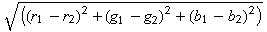
A Euclidean distance is the square root of the sum of the squared differences between the color of the first source and the color of the second source. A Euclidean distance is generally regarded as a well-known standard distance calculation.
The following example illustrates how the distance between a green point, indicated by a circle, and two other green points, indicated by a triangle and a square, is measured with a Euclidean calculation.
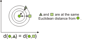
A Euclidean distance can be represented with the following formula, where:
|
|
Manhattan distance
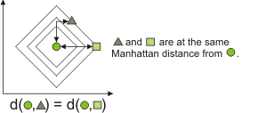
A Manhattan distance (also known as a City Block distance) is the sum of the absolute value of the differences between the color of the first source and the color of the second source. A Manhattan distance is generally considered the simplest distance calculation and is typically appropriate for calculating color distances between hue (H) bands in HSL. For example, using McolMatch() with an HSL color space, and calculating the distance between the zero (H) bands (McolControl() with M_BAND_MODE set to M_COLOR_BAND_0).
The following example illustrates how the distance between a green point, indicated by a circle, and two other green points, indicated by a triangle and a square, is measured with a Manhattan calculation.
A Manhattan distance can be represented with the following formula, where:

|
|
Note that in HSL the color's hue is stored as a separate component (H) represented as an angular position on a circular color disk. Therefore the distance between colors is equal to the smallest angular difference, rather than the absolute value of the difference.
Mahalanobis distance
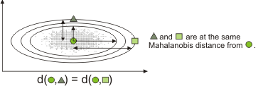
A Mahalanobis distance is calculated between the color of the first source and the covariance of the second source. If you are using McolDistance() and the second source is an image, the covariance of that image, rather than the color of each pixel, is used to calculate the distance. If you are using McolSetMethod(), the covariance of the color-sample is used. A Mahalanobis distance is generally regarded as a slower, though more robust distance calculation for elongated color-samples.
The following example illustrates how the distance between a green point, indicated by a circle, and two other green points, indicated by a triangle and a square, is measured with a Mahalanobis calculation.
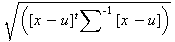
A Mahalanobis distance can be represented with the following formula, where:
|
|
The distance calculated for Mahalanobis, between a color and a distribution of colors (covariance), is similar to a Euclidean distance between the mean of the two colors, but weighted by the inverse of the covariance of the distribution. This implies that the more a color distribution varies in a direction within the color space, the less significant the distance is in that direction.
Since the covariance matrix of the second source is used, the second source should typically be a distribution of colors, such as an image, and not a single solid color (a color constant). However, if you provide a color constant as the second source, Mahalanobis behaves very much like Euclidean and will yield similar results.
Delta-E distance
A Delta-E color distance is similar to a Euclidean color distance, but has been generally adjusted for the LAB (CIELAB) color space. That is, MIL converts the color data to the native LAB range before performing a Euclidean-type color distance. You would therefore typically use Delta-E when working with CIELAB, as defined by the International Commission on Illumination (CIE).
Advanced CIE distance types
In addition to M_DELTA_E, MIL offers more specialized types of CIE color distances, which you can specify using McolSetMethod(). These types are recommended for advanced users dealing with minor color variances in industrial color difference evaluation.
These distance types follow the standards of the CIE, as specified in their technical report on Colorimetry (CIE 15:2004). Refer to this document for more information.
Choosing a distance type
Choosing the most appropriate distance type with which to calculate color distances depends on many factors, including the color space of your data, the background, and the particularities of your application. Typically, a Euclidean distance should be used for RGB and CIELAB color spaces, while a Manhattan distance should be used for HSL. A Mahalanobis color distance should be used when dealing with closely-related colors that are not expressed in HSL.
The following example illustrates an RGB source image of a grapefruit, which is to be used in a matching operation. Although for RGB colors a Euclidean distance is typically sufficient, in this case a Mahalanobis distance is preferable.
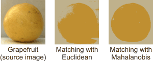
In the source image, the color of the background and some parts of the grapefruit are similar; this makes Mahalanobis yield better results, since the covariance of the image is used. The pixels of the grapefruit correspond roughly to a distribution of shades of yellow, therefore, with a Mahalanobis distance, shades of yellow are considered to be closer to the grapefruit than other colors. To illustrate this point, the following image (a plotting of the color histogram) shows two separate groups of pixels displayed in RGB; one group is from the image's background, and the other is from the grapefruit.
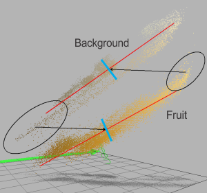
For each group of pixels (background and grapefruit), this image shows:
Encircled in black, on the left, are the background pixels that will match the grapefruit, being closer by Euclidean distance to the grapefruit's mean color. Encircled in black, on the right, are the grapefruit's pixels that will match the background, being closer by Euclidean distance to the background's mean color. However, with a Mahalanobis distance, any distance oriented parallel to the principal component (the red lines) will be scaled by the inverse of the standard deviation. Therefore, the encircled pixels will match with the correct group (background or grapefruit), yielding a better matching result.