Histogram equalization
A histogram equalization can be performed to obtain a more uniform distribution of the grayscale values in your image. For example, if the intensity distribution of an image results in a clump in one area of the grayscale range, there might be objects that are not easily distinguished because of their similarity in color. You might want to adjust the image's intensity distribution to solve this problem by giving it a more uniform (M_UNIFORM) distribution, using MimHistogramEqualize().
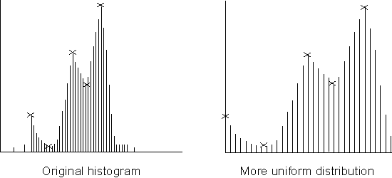
The MimHistogramEqualize() function first generates a histogram of the source image buffer. The histogram and a selected density function are then used to calculate a transformation LUT. If the destination buffer is an image, the transformation LUT is applied to the source buffer to produce the destination image. If the destination buffer is a LUT, the transformation LUT is copied into the destination LUT; this LUT can then be used to enhance the source image, either permanently (using MimLutMap()) or upon display (using MdispLut()). The transformation LUT can also be applied directly to images as they are being grabbed; to do so, first associate the LUT buffer with the digitizer, using MdigControl() with M_LUT_ID and then grab the image.
Adaptive histogram equalization
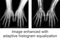
By calling MimHistogramEqualizeAdaptive(), you can enhance an image with a Contrast Limited Adaptive Histogram Equalization (CLAHE). In this case, you must allocate an adaptive histogram equalization context, using MimAlloc() with M_HISTOGRAM_EQUALIZE_ADAPTIVE_CONTEXT.
Adaptive histogram equalization is not available with MIL-Lite.
Unlike a conventional histogram equalization (MimHistogramEqualize()), which generates a histogram for the entire image as a whole, MimHistogramEqualizeAdaptive() partitions the specified image into a set of rectangular sections of equal size, referred to as tiles, and calculates histograms for each one. The multiple histograms, along with the specified equalization operation, are then used to transform the image and produce an enhanced version of it. Though this can take slightly longer than a conventional histogram equalization, it can help minimize the over-amplification of noise and the potential for saturation, particularly in images with inconsistent lighting where some sections are significantly brighter than others.
By default, MimHistogramEqualizeAdaptive() uses 8 tiles along the image's X- and Y-direction. The specified image is therefore processed as 64 congruent tiles. To modify this behavior, use MimControl() with M_NUMBER_OF_TILES_X and M_NUMBER_OF_TILES_Y.
Every tile of the image has its own histogram, and every histogram has a set of bins, each indicating the number of pixels with the same intensity. The maximum percentage of pixels that a bin can represent is limited, by default, to 1% of all the pixels in that tile. To modify the maximum percentage, use the M_CLIP_LIMIT control. This essentially limits the contrast. Exceeding values are distributed evenly among the tile's other histogram bins.
You can also modify the number of histogram bins for each tile, as well as the equalization operation to perform, using the M_HIST_SIZE and M_OPERATION controls. By default, MimHistogramEqualizeAdaptive() determines the number of histogram bins automatically according to the specified source image and performs a uniform-type of equalization.
Theoretically, the equalization can process each pixel and its neighborhood for every tile. To avoid this lengthy calculation, MimHistogramEqualizeAdaptive() actually performs a type of interpolation between the intensities of adjacent tiles, which drastically improves efficiency while only negligibly diminishing the quality of the transformed image. For more information about this, and other specifics regarding CLAHE, refer to "S. M. Pizer, E. P. Amburn, J. D. Austin, et al. Computer Vision, Graphics, and Image Processing: Adaptive Histogram Equalization and Its Variations . U.S.A.: Elsevier, 1986. 355-368.".
The following example demonstrates how to perform an adaptive histogram equalization: