Pattern matching algorithm (for advanced users)
- See also

 Availability
 Previous
- Next

Normalized grayscale correlation is widely used in industry for pattern matching applications. Although in many cases you do not need to know how the search operation is performed, an understanding of the algorithm can sometimes help you pick an optimal search strategy.
Normalized correlation
The correlation operation can be seen as a form of convolution, where the pattern matching model is analogous to the convolution kernel (see the Custom spatial filters section of Chapter 4: Advanced image processing). Ordinary (un-normalized) correlation is exactly the same as a convolution:

In other words, for each result, the N pixels of the model are multiplied by the N underlying image pixels, and these products are summed. Note, the model does not have to be rectangular because it can contain "don't care" pixels that are completely ignored during the calculation. When the correlation function is evaluated at every pixel in the target image, the locations where the result is largest are those where the surrounding image is most similar to the model. The search algorithm then has to locate these peaks in the correlation result, and return their positions.
Unfortunately, with ordinary correlation, the result increases if the image gets brighter. In fact, the function reaches a maximum when the image is uniformly white, even though at this point it no longer looks like the model. The solution is to use a more complex, normalized version of the correlation function (the subscripts have been removed for clarity, but the summation is still over the N model pixels that are not "don't cares"):
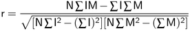
With this expression, the result is unaffected by linear changes (constant gain and offset) in the image or model pixel values. The result reaches its maximum value of 1 where the image and model match exactly, gives 0 where the model and image are uncorrelated, and is negative where the similarity is less than might be expected by chance.
In our case, we are not interested in negative values, so results are clipped to 0. In addition, we use r2 instead of r to avoid the slow square-root operation. Finally, the result is converted to a percentage, where 100% represents a perfect match. So, the match score returned by MpatGetResult() is actually:
Score = max(r, 0) 2 x 100%.
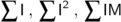
Note, some of the terms in the normalized correlation function depend only on the model, and hence can be evaluated once and for all when the model is defined. The only terms that need to be calculated during the search are:
This amounts to two multiplications and three additions for each model pixel.
The sums used to compute the correlation function can be retrieved using MpatGetResult(). The retrievable sums are the following:

The number of pixels N is also available using MpatGetResult(). The above sums are only available if they are saved in the result buffer using MpatControl() with M_SAVE_SUMS set to M_ENABLE. These sums can be used, for example, to assess the model or target intensity level and contrast.
Note that the correlation function calculated with the retrieved sums, will probably differ from the score returned by MpatGetResult(). Although the score is derived from the correlation function, it also depends on the first and last subsampling levels chosen, optimization schemes and subpixel interpolation.
On a typical computer, the multiplications alone account for most of the computation time. A typical application might need to find a 128x128-pixel model in a 512x512-pixel image. In such a case, the total number of multiplications needed for an exhaustive search is 2x512 2 x128 2 , or over 8 billion. On a typical computer, this would take a few minutes, much more than the 5 msec or so the search actually takes. Clearly, MpatFind() does much more than simply evaluate the correlation function at every pixel in the search region and return the location of the peak scores.
Hierarchical search
A reliable method of reducing the number of computations is to perform a so-called hierarchical search. Basically, a series of smaller, lower-resolution versions of both the image and the model are produced, and the search begins on a much-reduced scale. This series of subsampled images is sometimes called a resolution pyramid, because of the shape formed when the different resolution levels are stacked on top of each other.
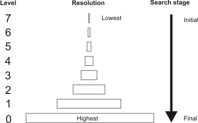
Each level of the pyramid is half the size of the previous one, and is produced by applying a low-pass filter before subsampling. If the resolution of an image or model is 512x512 at level 0, then at level 1 it is 256x256, at level 2 it is 128x128, and so on. Therefore, the higher the level in the pyramid, the lower the resolution of the image and model.
The search starts at low resolution to quickly find likely match candidates. It proceeds to higher and higher resolutions to refine the positional accuracy and make sure that the matches found at low resolution actually were occurrences of the model. Because the position is already known from the previous level (to within a pixel or so), the correlation function need be evaluated only at a very small number of locations.
Since each higher level in the pyramid reduces the number of computations by a factor of 16, it is usually best to start at as high a level as possible. However, the search algorithm must trade off the reduction in search time against the increased chance of not finding the pattern at very low resolution. Therefore, it chooses a starting level according to the size of the model and the characteristics of the pattern. In the application described earlier (128x128 model and 512x512 image), it might start the search at level 4, which would mean using an 8x8 version of the model and a 32x32 version of the target image.
To determine the default first and last resolution levels, use MpatInquire() with M_PROC_FIRST_LEVEL and M_PROC_LAST_LEVEL, respectively. If required, you can change the first and last resolution levels, using MpatControl() with M_FIRST_LEVEL and M_LAST_LEVEL to either a specific or the maximum possible level, repetitively. You can set the first resolution level to a specific value or you can have MIL automatically set the best first level, based on the model's size or its content.
When dealing with images without much fine detail, you should have MIL automatically select the first resolution level from the model's size (using M_AUTO_SIZE_BASED). This can provide a faster search, but fine details can be lost when dealing with larger images. In cases where fine details are present in larger target images, you should have MIL automatically select a first resolution level from the model's content (using M_AUTO_CONTENT_BASED). This intelligent analysis is typically slower, but can provide more robust results.
The logic of a hierarchical search accounts for a seemingly counter-intuitive characteristic of MpatFind(): large models tend to be found faster than small ones. This is because a small model cannot be subsampled to a large extent without losing all detail. Therefore, the search must begin at fairly high resolution (low level), where the relatively large search region results in a longer search time. Thus, small models can only be found quickly in fairly small search regions.
Note that the pyramidal representation of the buffer is generated each time MpatFind() is called. However, you can save the pyramidal representation of the buffer (generated when MpatFind() is called) in the result buffer, using MpatControl() with M_TARGET_CACHING. This pyramidal representation is re-used by consecutive calls to MpatFind() as long as the same result buffer is used and the image, search region, and model size are not modified.
Search region
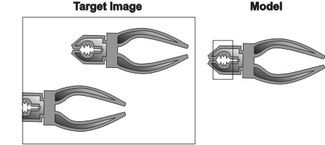
A zero-overscan technique is used to search for partially occluded occurrences near the border of the target image. However, this can lead to lower score and lower accuracy. In the example below, the left-most occurrence, which overlaps the border of the target image, would yield a lower score than the right-most occurrence.
Search heuristics
Even though performed at very low resolution, the initial search still accounts for most of the computation time if the correlation is performed at every pixel in the search region. On most models, match peaks (pixel locations where the surrounding image is most similar to the model, and correlation results are largest) are several pixels wide. These can be found without evaluating the correlation function everywhere. MpatPreprocess() analyzes the shape of the match peak produced by the model, and determines if it is safe to try to find peaks faster. If the pattern produces a very narrow match peak, an exhaustive initial search is performed. The search algorithm tends to be conservative; if necessary, force fast peak finding, using MpatControl() with M_FAST_FIND.
Using MpatControl() with M_EXTRA_CANDIDATES, you can set the number of extra peaks to consider. Normally, the search algorithm considers only a limited number of (best) scores as possible candidates to a match when proceeding at the most subsampled stage. You can add robustness to the algorithm, by considering more candidates, without compromising too heavily on search speed. In addition, you can use MpatControl() with M_COARSE_SEARCH_ACCEPTANCE to set a minimum match score, valid at all levels except the last level, to be considered as an occurrence of the model. This ensures that possible models are not discarded at lower levels, yet maintains the required certainty during the final level.
At the last (high-resolution) stage of the search, the model is large, so this stage can take a significant amount of time, even though the correlation function is evaluated at only a very few points. To save time, you can select a high search speed, using MpatControl() with M_SPEED. For most models, this has little effect on the score or accuracy, but does increase speed.
Subpixel accuracy
The highest match score occurs at only one point, and drops off around this peak. The exact (subpixel) position of the model can be estimated from the match scores found on either side of the peak. A surface is fitted to the match scores around the peak and, from the equation of the surface, the exact peak position is calculated. The surface is also used to improve the estimate of the match score itself, which should be slightly higher at the true peak position than the actual measured value at the nearest whole pixel.
The actual accuracy that can be obtained depends on several factors, including the noise in the image and the particular pattern of the model. However, if these factors are ignored, the absolute limit on accuracy, imposed by the algorithm itself and by the number of bits and precision used to hold the correlation result, is about 0.025 pixels. This is the worst-case error measured in X or Y when an image is artificially shifted by fractions of a pixel. In a real application, accuracy better than 0.05 pixels is achieved for low-noise images. These numbers apply if you select high-accuracy search, using MpatControl() with M_ACCURACY, in which case the search always proceeds to resolution level 0.
If you select medium accuracy (the default), the search might stop at resolution level 1, and hence the accuracy is half of what can be attained at level 0. Selecting low accuracy might cause the search to stop at level 2, so the accuracy is reduced by an additional factor of two (to about 0.2 pixel).