Using images acquired with a Bayer color filter
- See also

 Availability
 Previous
- Next

-
Determine the gamma correction exponents (optional). For information on how to calculate the exponents, see the Performing gamma correction subsection of this section.
-
Determine the white balancing coefficients (optional). For information on how to calculate the coefficients, see the White balancing your Bayer images subsection of this section.
-
Grab or load a Bayer image into your source buffer.
-
Apply the MIL Bayer filter on the image using MbufBayer(), including the white balancing coefficients and/or gamma correction exponents, if they are being used. To use the adaptive demosaicing algorithm, you must also add M_ADAPTIVE to the ControlFlag parameter.
-
Grab an image that is a uniform shade of gray. To do so, hold a flat, smooth, non-reflective object that is a uniform shade of gray in front of the camera so that the object occupies the camera's entire field of view. The shade of gray should not be too close to white (too saturated); otherwise, one or more of the color bands might be clipped during the grab to maximum saturation, and the imbalance between the bands cannot be properly observed.
Ensure that the image is grabbed under the same lighting conditions as subsequent source images. Note that it is unlikely that you will be able to grab an image whose pixels have the same red, green, and blue value.
-
Allocate a 3x1 (or 6x1 if gamma is used) MIL array of type M_FLOAT using MbufAlloc1d() or MbufAlloc2d().
-
Call MbufBayer(), using the gray image as the source image, and adding M_WHITE_BALANCE_CALCULATE to the ControlFlag parameter. This call calculates the three coefficients required to white balance the specified source image and writes them to the array.
Alternatively, you could fill an array with custom values, and then load these values (in the order described below) into the MIL array using MbufPut1d() or MbufPut2d().
-
Grab the image required for the Bayer conversion.
-
Call MbufBayer(), using the new source image and the MIL array with the white balance coefficients.
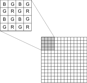
Cameras that feature a Bayer color filter can be used with MIL to provide a cost-effective method for grabbing color images: the camera grabs a single-band color-encoded image, and then you can convert it to a multi-band color image, using the MbufBayer() function. This conversion is called demosaicing. Bayer images are distinct from standard single-band images because of the color information contained in their pixels, which is extracted by the MbufBayer() function.
When grabbing from these cameras, each pixel quantifies only one of the color components of the image in the camera's field of view at the corresponding location. Within a group of 2x2 pixels, there are two pixels containing color information for the green component, and one pixel for each the red and blue components; Bayer images contain more green pixels because the human eye is more sensitive to this color. The pixels are arranged in the following pattern: green pixels are always diagonal to each other, as are the red and blue pixels.
The MbufBayer() function can also perform gamma correction and white balancing on the Bayer image before the demosaicing process, and color correction after the demosaicing process. Gamma correction changes the overall brightness and color saturation of an image so that the midtones appear more realistic on your display device; gamma correction effectively adjusts an image to compensate for the non-linear relationship between a pixel's value and its displayed intensity on your display device. White balancing adjusts an image for color variations that were introduced by the lighting conditions when the image was grabbed; MbufBayer() converts pixels that represent white so they appear as close to white as possible, and adjusts other pixels accordingly. Color correction adjusts an image for color artifacts that are introduced during the demosaicing operation and that appear on the transition edges of the image. Gamma correction, white balancing, and color correction are discussed in greater detail later in this section.
Note that if the scale of the image is changed (using MdigControl() with M_GRAB_SCALE...) to a value other than 1 prior to grabbing a Bayer image, the Bayer image will not be converted properly; some of the Bayer pattern is lost during the scaling process, rendering color recovery impossible.
Using MIL to convert the image
The steps below describe, in general, how to convert a Bayer image using MIL:
Below is an example of how to grab a Bayer image and convert it to a 3-band color image. This example also shows how to correct the white balance, which will be discussed later in this section.
How the Bayer image gets converted
Bayer images are arranged in groups of 2x2 pixels. Each group contains one blue pixel, one red pixel, and two green pixels; the values of which are used in calculating the corresponding bands of the destination pixels. Your camera will grab an image with one of the following four patterns:
.png)
You must specify the pattern that is used by your camera when calling MbufBayer(). Since the green pixels are always diagonal to each other, specifying the starting two pixels of the pattern defines the pattern uniquely. Consult your camera's documentation or contact the manufacturer if you are unsure; the Bayer image will not be converted properly if you specify the wrong pattern. If you cannot obtain information regarding the pattern of your camera, try all of the MbufBayer() function's supported patterns to find the correct one.
Once you have specified the Bayer pattern of your camera, you must consider which demosaicing algorithm to use to convert a single-band Bayer color-encoded image to a multi-band color image. There are currently two from which you can choose from: the bilinear interpolation demosaicing algorithm and the adaptive demosaicing algorithm.
Bilinear interpolation algorithm
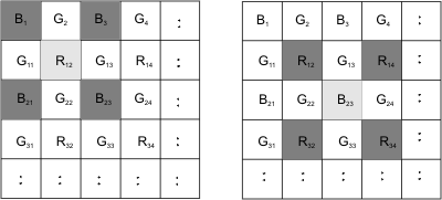
When using the bilinear interpolation algorithm, the value of a source pixel is used in the corresponding band of its destination pixel. The two remaining color bands use the average value of the source pixel's corresponding neighbors. If the source pixel is green, then the average value for the remaining two components (red and blue) is based on two neighboring pixels.
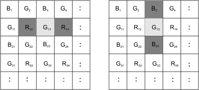
If the source pixel is either red or blue, the average value for the remaining two components is based on four neighboring pixels.
Note that if the source pixel is on an edge of the image, MIL will use as many neighbors as possible when determining the average pixel value for the remaining components.
Regardless of the destination buffer format, MIL converts the Bayer image first to RGB, and then to the format of the destination buffer.
This is the default demosaicing algorithm used by MbufBayer().
Adaptive algorithm
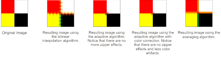
The bilinear demosaicing algorithm is simple, fast, and does an effective job of demosaicing the Bayer images. However, since it uses only the neighborhood averages to determine the pixel values, details are sometimes lost and sporadic artifacts are introduced. To minimize image artifacts, such as the zipper effect and false colors, you can use the adaptive demosaicing algorithm to convert your images.
The adaptive demosaicing algorithm analyzes the surrounding neighborhood of the source pixel and assigns weights to its neighbors. MIL then uses these weights in the calculation of the destination pixel value, depending on the neighbor's relevancy to the source pixel.
To use the adaptive demosaicing algorithm, add M_ADAPTIVE to the ControlFlag parameter.
Average algorithm
The average algorithm is the fastest demosaicing algorithm. The average algorithm uses a 2x2 neighborhood kernel to perform the demosaicing. When using this algorithm the zipper effect is minimal, but the image is shifted by half a pixel to the left and by half a pixel upwards and some false colors can be introduced.
To use the average demosaicing algorithm, add M_AVERAGE_2X2 to the ControlFlag parameter.
Performing color correction
Sometimes grabbed images appear with a color fringe on transition edges. To minimize these color artifacts on the edges, you can perform a color correction on the image during the Bayer conversion.
Color correction can only be used in conjunction with the adaptive demosaicing algorithm and is designed to produce very good looking vertical and horizontal edges. For best visual results, you should combine M_ADAPTIVE and M_COLOR_CORRECTION together.
The following compares the results of the two demosaicing algorithms and the effect of color correction.
Performing gamma correction
For typical machine vision processing applications, an image should not be gamma corrected; however, it can be useful to perform gamma correction for display purposes. There is typically a non-linear relationship between a pixel's value and its displayed intensity on your display device. Therefore, images can look either bleached out or too dark. You can compensate for the non-linear output of your display device by performing gamma correction. You should pass positive exponents in the range of 0.0 to 1.0 (most commonly, 0.45) for the red, green, and blue band in the fourth, fifth, and sixth elements of the MIL array buffer, respectively. MbufBayer() performs gamma correction on the raw RGB values of your image before performing white balancing and demosaicing.
White balancing your Bayer images
Sometimes grabbed images appear with "the wrong colors". This is due primarily to color distortions introduced by the light source or lighting conditions. You can correct such distortions by performing white balancing on the image. MbufBayer() uses the gray world assumption algorithm to perform white balancing.
The steps below show how to white balance Bayer images using the MbufBayer() function:
When MbufBayer() calculates the coefficients, the three white balancing coefficients, a, b, and c, are calculated and written to the array as the first, second, and third values, respectively. These coefficients are for a given lighting condition, and calculated such that given an image of a flat gray surface in that lighting:
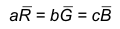
where R, G, and B with macrons (¯) are the average values of the red, green, and blue color components, respectively. When source images are converted, the color components of each pixel are multiplied by their corresponding coefficient. Regardless of the destination buffer format, white balancing is performed on the gamma corrected RGB values (if gamma correction is performed at all).