Adjusting the intensity distribution

• See also
Reference:
MbufAlloc1d MbufControl MdigControl MdispLut MgenLutRamp MimAlloc MimControl MimHistogramEqualize MimHistogramEqualizeAdaptive MimLutMap MimMorphic MimRemap
Availability
Available in MIL-Lite with restrictions


Available in MIL
Previous
Next

There are two ways to adjust the intensity distribution of an image:

Window leveling

Window leveling takes a range of pixel values in the source image and linearly maps these values to a different range in the destination image.

By stretching the range of values actually present in an image to the full range available, window leveling allows you to use all available intensities. Window leveling is especially useful when examining 10- or 12-bit images that have been grabbed into 16-bit images so that the image can occupy all of the available intensity range.

When using MIL, you will sometimes be limited to using 8-bit image buffers. If your images have a greater bit depth, you can use window leveling to map your images to an 8-bit range. For example, to convert a 10-bit image into an 8-bit image, you can set the destination to an 8-bit image buffer and set the output range of the window leveling as 0 to 255.

Window leveling using MimRemap()

The function MimRemap() performs a point-to-point linear remapping of pixel values, from the source range to the destination range, according to the specified mode. For the source range, you can specify to use the minimum and maximum values supported by the source image buffer (M_FIT_SRC_RANGE), or you can have MIL find the pixel value extremes of the source image (M_FIT_SRC_DATA). In either case, source values are mapped to the destination buffer's specified range of possible values. To control the pixel value range of the source or destination buffer, use MbufControl() with M_MIN and M_MAX.

You can choose to keep the destination range centered to zero (M_CENTERED). In the centered case, the values are remapped such that the value zero in the source buffer maps to the value zero in the destination buffer.

You can use MimRemap() to compress or expand an image to a different bit depth, since the bit depth can differ between the specified source and destination image buffers. For example, you can use MimRemap() with M_FIT_SRC_RANGE to convert down to an 8-bit depth for display purposes or to be able to use analysis modules that only accept 8-bit input.

The table below shows the formulas used by MimRemap(), for both the centered and non-centered cases.

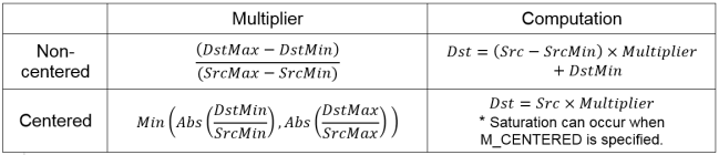
Note that, in the centered case, some exceptions to the multiplier calculation apply. If both SrcMax and DstMax are less than zero, the multiplier is DstMin/SrcMin . If both SrcMin and DstMin are greater than or equal to zero, the multiplier is DstMax/SrcMax .

MimRemap() is not available with MIL-Lite.

Window leveling using MimLutMap()

You can use a LUT when performing window leveling. In this case, use MimLutMap() after generating a LUT and associated ramp. You can choose specific intensity ranges within both the source and destination images.

The image below illustrates the effects of window leveling using MimLutMap().

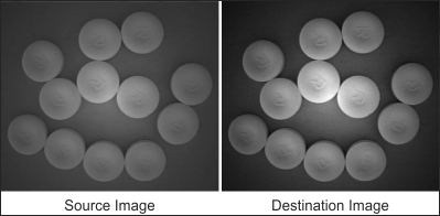
To implement window leveling using MimLutMap(), you must first allocate a LUT buffer using MbufAlloc1d() with a size equivalent to the maximum possible value in the source image. Generate a ramp for the LUT using MgenLutRamp(), specifying the StartValue and EndValue as the required range of the destination image buffer. Finally, map the source image buffer through the LUT using MimLutMap().

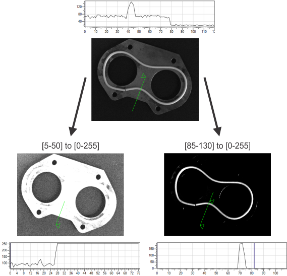
You can use window leveling if you want to improve the contrast in your images and highlight distinct areas. Stretching a particular range of values in an image will make some features of the image closely resemble other features or the background, which can be useful for analysis. You can also stretch a portion of an image's intensity range to see certain details (for example, in medical x-ray applications, various tissue types occupy different value ranges). The following image illustrates how you can highlight different features using window leveling:

The following example demonstrates how to perform window leveling using a LUT.

/* Calculate the minimum and maximum pixel values of the source image. */
MIL_ID MilStatContext = MimAlloc(MilSystem, M_STATISTICS_CONTEXT, M_DEFAULT, M_NULL);
MIL_ID MilStatResult = MimAllocResult(MilSystem, M_DEFAULT, M_STATISTICS_RESULT, M_NULL);
MimControl(MilStatContext, M_STAT_MAX, M_ENABLE);
MimControl(MilStatContext, M_STAT_MIN, M_ENABLE);


MimStatCalculate(MilStatContext, MilOriginalImage, MilStatResult, M_DEFAULT);
MimGetResult(MilStatResult, M_STAT_MAX + M_TYPE_MIL_INT, &ImageMaxValue);
MimGetResult(MilStatResult, M_STAT_MIN + M_TYPE_MIL_INT, &ImageMinValue);

//. . .

/* Allocate a LUT buffer */
MbufAlloc1d(MilSystem, 255 + 1, 8 + M_UNSIGNED, M_LUT, &MilLut);

/* Generate a LUT with a full range ramp. */
MgenLutRamp(MilLut, ImageMinValue, 0.0, ImageMaxValue, 255.0);
MimLutMap(MilOriginalImage, MilResultImage, MilLut);

//. . .

For a more interactive example, see the following example.

Window leveling using MimMorphic()

To perform window leveling on a pixel neighborhood basis, rather than point-to-point, use MimMorphic() with M_LEVEL. This operation finds the pixel value extremes in a specified pixel neighborhood, then maps this range to the full range available in the total image. Similar to using MimRemap() with M_FIT_SRC_DATA, the MimMorphic() operation is like an adaptive window leveling, since only local pixel extremes are calculated.

MimMorphic() is not available with MIL-Lite.

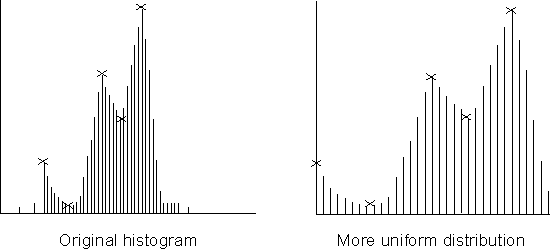
Histogram equalization

A histogram equalization can be performed to obtain a more uniform distribution of the grayscale values in your image. For example, if the intensity distribution of an image results in a clump in one area of the grayscale range, there might be objects that are not easily distinguished because of their similarity in color. You might want to adjust the image's intensity distribution to solve this problem by giving it a more uniform (M_UNIFORM) distribution, using MimHistogramEqualize().

The MimHistogramEqualize() function first generates a histogram of the source image buffer. The histogram and a selected density function are then used to calculate a transformation LUT. If the destination buffer is an image, the transformation LUT is applied to the source buffer to produce the destination image. If the destination buffer is an LUT, the transformation LUT is copied into the destination LUT; this LUT can then be used to enhance the source image, either permanently (using MimLutMap()) or upon display (using MdispLut()). The transformation LUT can also be applied directly to images as they are being grabbed; to do so, first associate the LUT buffer with the digitizer, using MdigControl() with M_LUT_ID and then grab the image.

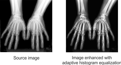
Adaptive histogram equalization

For a more refined histogram equalization, use MimHistogramEqualizeAdaptive(), which enhances an image using a contrast limited adaptive histogram equalization (CLAHE). In this case, you must allocate an adaptive histogram equalization context, using MimAlloc() with M_HISTOGRAM_EQUALIZE_ADAPTIVE_CONTEXT.

Adaptive histogram equalization is not available with MIL-Lite.

Unlike a conventional histogram equalization (MimHistogramEqualize()), which generates a histogram for the entire image as a whole, MimHistogramEqualizeAdaptive() partitions the specified image into a set of rectangular sections of equal size, referred to as tiles, and calculates histograms for each one. The multiple histograms, along with the specified equalization operation, are then used to transform the image and produce an enhanced version of it. Though this can take slightly longer than a conventional histogram equalization, it can help minimize the over-amplification of noise and the potential for saturation, particularly in images with inconsistent lighting where some sections are significantly brighter than others.

By default, MimHistogramEqualizeAdaptive() uses 8 tiles along the image's X- and Y-direction. The specified image is therefore processed as 64 congruent tiles. To modify this behavior, use MimControl() with M_NUMBER_OF_TILES_X and M_NUMBER_OF_TILES_Y.

Every tile of the image has its own histogram, and every histogram has a set of bins, each indicating the number of pixels with the same intensity. The maximum percentage of pixels that a bin can represent is limited, by default, to 1% of all the pixels in that tile. To modify the maximum percentage, use the M_CLIP_LIMIT control. This essentially limits the contrast. Exceeding values are distributed evenly among the tile's other histogram bins.

You can modify the number of histogram bins for each tile, as well as the equalization operation to perform, using the M_HIST_SIZE and M_OPERATION control types, respectively. By default, MimHistogramEqualizeAdaptive() determines the number of histogram bins automatically according to the specified source image, and performs a uniform-type of equalization.

Theoretically, the equalization can process each pixel and its neighborhood for every tile. To avoid this lengthy calculation, MimHistogramEqualizeAdaptive() actually performs a type of interpolation between sample pixel regions of adjacent tiles to determine pixel value results, which significantly improves efficiency, while only negligibly diminishing the quality of the transformed image. For more information about this, and other specifics regarding CLAHE, refer to "S. M. Pizer, E. P. Amburn, J. D. Austin, et al. Computer Vision, Graphics, and Image Processing: Adaptive Histogram Equalization and Its Variations . U.S.A.: Elsevier, 1986. 355­-368.".

The following example demonstrates how to perform an adaptive histogram equalization: