Controlling a JPEG compression
- See also

 Availability
 Previous
- Next

This section provides a brief overview of the JPEG lossless and lossy algorithms and of the controls you have over these algorithms. In general, you should only change these controls if you are familiar with the algorithm you are using. For detailed information about the JPEG lossless and lossy algorithms, see Information technology -- Digital compression and coding of continuous-tone still images: Requirements and guidelines, which is available from the International Standards Organization (http://www.iso.ch). For techniques to use to improve compression operations, see the Improving results section later in this chapter.
Note that during development and at runtime, compression support is reliant upon the presence of a compression/decompression package license. This license is only included by default with the development dongle for the full version of MIL. In other cases, this license must be purchased separately.
JPEG lossless
The JPEG lossless algorithm is basically a two-step process. First, predictive coding is performed on the image. Then, the result is Huffman encoded.
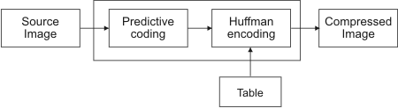
Predictive coding
Predictive coding is based on the fact that adjacent pixels in an image generally have similar values. Therefore, the value of a pixel can be "predicted" from the values of its neighbor(s). The difference between the original value of the pixel and the predicted value requires fewer bits to store than the original pixel value.
MIL supports three types of predictive coding: predictor #0 (no predictor), predictor #1 (the "pixel-to-the-left" predictor), and predictor #2 (the "pixel-above" predictor). By default, MIL uses the pixel-to-the-left to predict values, which is suitable for most images. In some applications, you might prefer to use the pixel-above predictor. You can also specify no predictor (predictor #0), but note that in this case, the values after predictive coding will be the same as the original values. This predictor can be useful if you have developed your own algorithm to take the place of predictive coding and only need your images Huffman encoded. Note that you must implement your own algorithm to use one of the other "predictors" supported by the JPEG lossless algorithm. You can use MbufControl() with the M_PREDICTOR control type to specify the predictor.
Huffman encoding
After an image has been predictive coded, Huffman encoding assigns a variable-length "code word" to each value. This code is based on the number of bits by which adjacent values differ. Values are assigned code words according to a DC Huffman table. You can use the default DC Huffman table or you can create your own table. If you want to use your own table, see the Working with tables section later in this chapter.
JPEG lossy
The JPEG lossy algorithm is outlined below. First the source image must be in the correct format before it can be compressed. Although the JPEG algorithm requires signed source data, the algorithm accepts both signed and unsigned data. Initially the algorithm internally treats all data as unsigned. Then a computational shift is performed to set all the values to signed.
After the computational shift, a color conversion is performed if the source and destination buffers are in different formats, for example an RGB source buffer and a YUV destination buffer. Note that conversion to YUV introduces some loss.
Afterwards, each 8x8 block of the image is represented in its frequency domain through a discrete cosine transform, resulting in 1 DC and 63 AC values. Each block is then quantized and Huffman encoded.
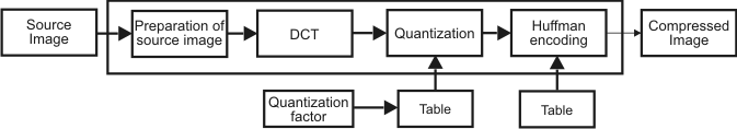
Quantization divides each of the 64 values in a block by a specified value, according to a quantization table. After each block is quantized, Huffman encoding assigns a variable-length "code word" to each value. Each DC value in a block is assigned a code word according to a DC Huffman table. The AC values are assigned a code word according to an AC Huffman table. You can control a JPEG lossy compression by using your own quantization and/or Huffman tables.
Restart markers
When an image is compressed, MIL adds restart markers to the bit-stream of the compressed image. A restart marker is a special code that signifies that the encoded bit-stream has been padded to the next byte boundary before the encoding process was restarted. Restart markers can be useful if you are transmitting the compressed image over a medium that is susceptible to errors. If an error does occur and there are no restart markers, the error will propagate and affect subsequent data. However, if there are restart markers, the error will be confined to the data between markers.
By default, MIL places restart markers after a certain number of rows of data have been encoded (for lossless compressions) or after a certain number of 8x8 blocks of data have been encoded (for lossy compressions). If necessary, you can use MbufControl() with the M_RESTART_INTERVAL control type to change the number of rows or blocks between restart markers.
For a lossy compression with a high compression ratio, too many restart markers can significantly increase the size of the compressed image. In this case, you might want to increase the number of blocks between restart markers, especially if you are not transmitting the image over a noisy medium. In fact, if you are sure that the transmission medium is not noisy, you might want to set the restart interval to 0, that is, not use restart markers. This will increase the compression ratio, as well as reduce the time required to decompress the image.