JPEG2000

---

• See also
User Guide:
Improving results Working with tables
Reference:
MbufControl MbufInquire
Availability
Available in MIL-Lite with restrictions


Available in MIL
Previous
Next

This section provides a brief overview of the JPEG2000 lossy and lossless algorithms and the control you have over these algorithms. Everything applicable to lossy compression is applicable to lossless compression, unless otherwise stated. In general, you should only change compression controls if you are familiar with the algorithm (except for the quantization factor, which you can change without in-depth knowledge, using MbufControl() with M_Q_FACTOR). For techniques to use to improve compression operations, see the Improving results section later in this chapter. For more detailed information about the JPEG2000 algorithm, see http://www.jpeg.org.

Note that during development and at runtime, compression support is reliant upon the presence of a compression/decompression package license. This license is only included by default with the development dongle for the full version of MIL. In other cases, this license must be purchased separately.

There are two fundamental differences between the JPEG2000 and regular JPEG compression algorithms. The first is the use of a discrete wavelet transform (DWT), instead of a discrete cosine transform. The second is the use of arithmetic encoding instead of Huffman encoding as the entropy encoding technique; arithmetic encoding reduces the number of bits required to encode data, based on how frequently that data occurs in the image.

When compared to regular JPEG compression, JPEG2000 supports much higher ratios of compression without compromising image quality. Note however, that JPEG2000 is best suited for archiving purposes because of the processing time required to compress and decompress images; therefore, JPEG2000 can be used for grabbing, but it presents a risk of missing frames.

When compressing images with the JPEG2000 algorithm, MIL supports:

Note that MIL does not support the following JPEG2000 features:

The JPEG2000 compression consists of the following steps:

Preparation of source image

Although the JPEG2000 algorithm requires signed source data, the algorithm accepts both signed and unsigned data. Initially the algorithm internally treats all data as unsigned. Then a computational shift is performed to set all the values to signed.

After the computational shift, a color conversion is performed if the source and destination buffers are in different formats, for example an RGB source buffer and a YUV destination buffer. Note that conversion from RGB to YUV naturally introduces some loss.

Discrete wavelet transform (DWT)

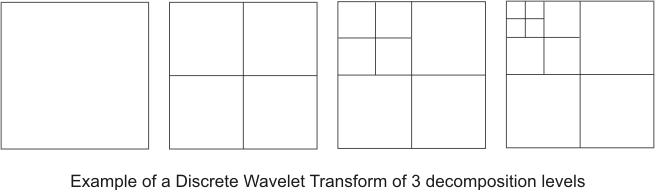
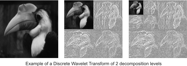
After preparation of the source image, a lossy or lossless discrete wavelet transform (DWT) is applied to the image. The discrete wavelet transform both subsamples and spatially filters the image. Depending on the type of compression, the DWT uses one of two sets of filters: for lossy compression, a Daubechies 9-tap/7-tap filter is used, while a 5-tap/3-tap filter is used for lossless compression. The DWT subsamples and then separates the data into high frequency areas and low frequency areas; these areas are referred to as sub-bands. Each iteration, which consists of one pass of both the high and low frequency filters in both the horizontal and vertical directions, results in four sub-bands. Subsequent iterations of the transform are always applied on the top-left (low frequency) sub-band. MIL refers to each iteration of the DWT as a decomposition level.

The default number of decomposition levels is 5, unless the width or the height of the image is less than or equal to 16 pixels; in which case, the number of decomposition levels is chosen so that the width or the height of the 4 smallest sub-bands of the image is 1 pixel. You can override the default using MbufControl() with M_DECOMPOSITION_LEVEL. For example, if your original image is 1024x768, by default, the number of decomposition levels is 5, and the size of the 4 smallest sub-bands is 32x24. If you set the M_DECOMPOSITION_LEVEL control type to 6, then the size of the smallest sub-bands would be 16x12. The largest number of decomposition levels is the one that yields a width or a height of 1 pixel for the 4 smallest sub-bands. After allocating the image buffer, you can inquire the number of decomposition levels that will be used, using MbufInquire() with M_DECOMPOSITION_LEVEL.

After the wavelet transform, each pixel in the original image becomes a wavelet coefficient. There will always be as many wavelet coefficients as there were pixels in the original image.

After the wavelet transform is applied, MIL no longer considers the data as an image.

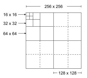
The larger sub-bands are further segmented into smaller regions, referred to as code-blocks. Smaller sub-bands are not segmented, and each contains one code-block. For example, if 64x64 code-blocks are used, the sub-band that is 128x128 contains four code-blocks, while the sub-bands that are 64x64, 32x32, and 16x16 each contain one code-block, as illustrated in the diagram below.

Segmentation optimizes compression by grouping areas with similar values; when the values to compress are similar, the result is a better compression ratio. Segmentation also optimizes access to Host memory, thereby improving the performance of the quantization (for JPEG2000 lossy compression), bit-plane decomposition, and arithmetic encoding steps in the algorithm.

Quantization

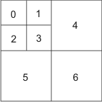
During JPEG2000 lossy compression, the wavelet coefficients contained in each code-block are quantized based on both the sub-band in which they fall, and an entry in the quantization table. Quantization multiplies each wavelet coefficient by its sub-band's corresponding entry, the quantization coefficient, in the table. The sub-band's rank in significance, which is illustrated below, determines which entry in the quantization table is used. Note that the top-left sub-band is the most significant.

JPEG2000 lossless compression does not use the quantization step.

MIL automatically determines the values for the quantization table based on the number of sub-bands resulting from the DWT transform; that is, all images of the same depth that have five decomposition levels will use the same quantization table. The first entry (for sub-band 0) always has the largest quantization coefficient.

When you adjust the quantization factor (using MbufControl() with M_Q_FACTOR), MIL scales all the quantization coefficients in the quantization table according to the specified factor. If you want more control, you can pass your own custom quantization table. To establish good values for a custom quantization table, you can inquire the default quantization coefficients. For more information, see the Working with tables section later in this chapter.

Bit-plane decomposition

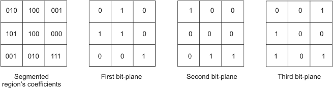
After the wavelet coefficients are multiplied by the quantization coefficients, the code-blocks are decomposed into bit-planes. A bit-plane contains the nth bit of all the multiplied wavelet coefficients that occupy a specific code-block. Decomposition into bit-planes is necessary for arithmetic encoding and post-processing.

A specific code-block might not have the same number of bit-planes as another code-block. Decomposition starts from the most-significant non-zero bit-plane of a code-block, and all subsequent bit-planes are decomposed, even eventual zero bit-planes. For example, the code-block in the diagram below contains coefficients that are 3 bits, and therefore will be decomposed into 3 bit-planes.

Arithmetic encoding

The bit-planes are then passed to the arithmetic encoder. The arithmetic encoder analyzes the bit-plane data to find redundancies, in other words, patterns of bits that occur frequently in the bit-planes. Using this information, the arithmetic encoder replaces repeating bit patterns, also called symbols, by shorter bit sequences. The more often a symbol occurs in the bit-plane data, the fewer bits into which that symbol will be coded.

During lossless compression, the arithmetic encoder processes each bit-plane to produce a continuous bit-stream. Since arithmetic encoding is the final stage of compression, this bit-stream is actually the compressed image.

During lossy compression, the arithmetic encoder produces several independent bit-streams; the post-processing step determines which bit-streams are concatenated in the final image.

Post-processing

Once the most-significant bit-plane of a code-block is encoded, its size in bytes is stored in memory, and MIL calculates how much error would be present in the decompressed image if the remaining bit-planes, for that code-block, were not arithmetically encoded.

Once the second most-significant bit-plane of the code-block is arithmetically encoded, MIL calculates the error introduced in the decompressed image if only the first two bit-planes were compressed. As each remaining bit-plane is encoded, MIL repeats the same calculation until all the bit-planes have been processed.

As an example only, the values in the following table represent the amount of distortion (error) with respect to the size in bytes of the encoded bit-planes of one code-block.

Bit-plane (in order of significance)	Compressed size in bytes	Distortion
1	5	58817925.11
2	54	34495584.39
3	159	11160557.81
4	296	2633195.13
5	436	594555.28
6	574	94112.98
7	717	21139.81
8	863	4080.74
9	980	0.00

Then, the best compromise between decompressed image quality and requested size in bytes (using MbufControl() with M_TARGET_SIZE) is determined. Any encoded bit-planes that are not required are discarded after the best compressed image is determined for the specified size. The remaining encoded bit-planes are then concatenated in the final image.

Determining an appropriate target size will require some trial and error, but a logical guess can be calculated by dividing the image's original size, in bytes, by the required compression ratio. For example, if you want to compress a 256-byte image by a factor of 16:1, you would specify a target size of 16 bytes.

Post-processing is not performed in JPEG2000 lossless, and none of the encoded bit-planes are discarded; therefore, you cannot specify a target buffer size when performing a lossless compression.