Working with 3D
- See also

 Availability
 Previous
- Next

-
Pass a 3D geometry object to the functions that support them to limit the processing region. To do so, allocate a 3D geometry object (using M3dgeoAlloc() with M_GEOMETRY), define the geometry's shape (using the appropriate function in the 3D Geometry module, or obtained as a result from another 3D image processing function), and then pass the 3D geometry object to the 3D function.
-
Copy the points of interest into a separate container and then use this container. To copy the points of interest, allocate a 3D geometry object, define the geometry's shape, and then use M3dimCrop() to crop points that are inside/outside the specified geometry object. M3dimCrop() can also perform cropping in-place (that is, the source container is the same as the destination container) without any reallocation if the resulting cropped point cloud is forced to have the same organizational structure as the source (M_SAME).
-
Mask unwanted points using a calibrated mask image buffer. To do so, use M3dimCrop(); 3D points projected onto 0-valued pixels in the specified calibrated mask image buffer are not kept in the resulting point cloud.
-
Change the data in the confidence component of a container to mask out unwanted regions. To do so, inquire the confidence component's MIL identifier using MbufInquireContainer() with M_COMPONENT_ID, and then pass the identifier of the component to MIL functions that work on image buffers to create the mask. For example, you can use the component with MbufCopyCond(), MIL image processing functions (such as MimArith()), or draw into the component using the 2D graphics functions (Mgra...()). Values set to 0 in the confidence component (M_COMPONENT_CONFIDENCE) cause the corresponding coordinates in the range component to be ignored.
-
Allocate a transformation matrix object using M3dgeoAlloc().
-
Generate the required transformation coefficients using M3dgeoMatrixSetTransform() or M3dgeoMatrixSetWithAxes(). Alternatively, you can copy a resulting matrix from another MIL 3D module (for example, the 3D Metrology or 3D Registration module) into the transformation matrix object.
-
Apply the transformation matrix to the 3D points using M3dimMatrixTransform().
The MIL 3D modules (M3d...) support display, analysis, and processing of 3D data of a scene. The 3D data can either be a point cloud or a depth map. A point cloud is a collection of data points, each with X-, Y-, and Z-coordinate values, and represents an object or scene in 3D space. A depth map is an image where the gray value of a pixel represents its depth in the world.
You can perform arithmetic and statistical operations, as well as comparative measurements between point clouds, depth maps, and 3D geometries. For example, you can fit a 3D geometry to a point cloud or depth map and calculate distances between points and the fitted surface.
You can scale, rotate, and translate 3D data, compute 3D profiles to examine a cross-section of data, and merge multiple point clouds or perform pairwise registration between point clouds. You can also sample a subset of points or reconstruct surfaces (meshes) for point clouds.
You can grab point clouds from a 3D sensor or generate point clouds from a laser line profiling setup. You can also load point clouds from PLY and STL files, or create them manually in your application.
3D data containers and grabbing
Typically, MIL 3D functions work with 3D data stored in a MIL container. A MIL container is a MIL object that contains buffers, called its components. You allocate a container using MbufAllocContainer().
To grab 3D data from a 3D sensor, you should pass a container to MdigGrab(), MdigProcess(), or MdigGrabContinuous(). These functions will automatically allocate components in the container appropriate for the data being transmitted from the 3D sensor.
Each component of a 3D container stores a different type of information about the 3D scene. The type of data stored in a component is typically set automatically; if not, you must specify it using MbufControlContainer() with M_COMPONENT_TYPE. Typically, respective positions in each component correspond to information about the same position in the scene.
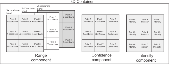
A 3D container has either a range component or a disparity component. A range component stores coordinates of points, or a depth map. A disparity component stores depth information grabbed from a stereoscopic camera. Typically, a 3D container also has a confidence component that stores whether each point should be used or ignored (for example, a point might be invalid because it was occluded during acquisition). The container can also have other components, such as an intensity component that stores the intensity or color of the points.
3D data in a container can be organized or unorganized. Organized 3D data is typically stored in components that are buffers with several rows; it is assumed that points close to each other in 3D space are also close to each other in the components (although not necessarily adjacent). Unorganized 3D data is stored in components that are buffers with a single row; the position of the points in the components has no meaning. For more information on point cloud organization, see the Organized and unorganized point clouds subsection of the Working with points in a point cloud section of Chapter 32: 3D image processing.
For more information on grabbing from devices that transmit 3D data in a format that is compliant with an industry standard (such as GigE Vision or GenICam), see the Working with compliant cameras section of Chapter 36: Grabbing from 3D sensors. Note that some 3D sensors transmit data in a non-compliant format. In this case, see the Working with non-compliant cameras section of Chapter 36: Grabbing from 3D sensors.
Converting 3D data for processing and 3D display
Although you can grab 3D data in many formats, you can only process and/or display 3D data if it is in a MIL 3D-processable or 3D-displayable format, respectively. You can inquire if a container is 3D-processable or 3D-displayable using MbufInquireContainer() with M_3D_PROCESSABLE or M_3D_DISPLAYABLE. If it isn't, you can convert it to a 3D-processable or 3D-displayable container using MbufConvert3d() (if the 3D data is in a format that is compliant with an industry standard). You can also use this function to convert a fully-corrected depth map image buffer to a 3D-processable or 3D-displayable point cloud container.
Before converting a 3D container using MbufConvert3d(), the 3D settings of the range or disparity component must be set correctly. These settings identify how 3D data is stored in the container (such as what scaling must be applied in each axis direction for the data to be natively calibrated). If your 3D sensor is configured to transmit this information, these settings will be set automatically during acquisition. Otherwise, you must set the 3D settings of the range or disparity component manually using MbufControlContainer() with settings from the table For specifying settings useful with components that store 3D data.
3D displays, and some 3D processing functions, support fully-corrected depth maps stored in image buffers. You cannot use the range component of a container as though it were a fully-corrected depth map image buffer; you must project the 3D data in the container to a fully-corrected depth map image buffer using M3dimProject(). If the range component stores a depth map in a specific format, you can convert the container to a fully-corrected depth map image buffer using MbufConvert3d().
For more information, see the Preparing a container for display or processing section of Chapter 35: 3D Containers.
Displaying 3D data
To display 3D data in 3D, you must first allocate a 3D display using M3ddispAlloc(). You can then select a 3D-displayable container or a fully-corrected depth map image buffer to the 3D display, using M3ddispSelect(). If you pass a container that is not in a 3D-displayable format, MIL will try to compensate by converting it internally. If this is not possible, an error will be generated.
Once a 3D display is shown in a window, you can look at the 3D data in the 3D display from different angles, either interactively using the mouse and keyboard or by manually specifying the required view using M3ddispSetView(). For more information, see the Manipulating the view section of Chapter 37: 3D Display and graphics.
You can also annotate the display with 3D graphics. To do so, inquire the 3D display's internal 3D graphics list using M3ddispInquire() with M_3D_GRAPHIC_LIST_ID, and then use the functions of the M3dgra...() module to draw into this 3D graphics list. For more information, see the Annotating the 3D display section of Chapter 37: 3D Display and graphics.
Processing 3D data
3D processing and analysis functions can work on MIL 3D-processable containers. Some can work on fully corrected depth map image buffers.
Calibration
When working with point cloud containers and/or 3D geometry objects, you do not associate them with a calibration context; all source data is treated as if it is natively calibrated. That is, a point cloud or geometry's coordinates are expected to be real world values. To work with a depth map with the 3D modules, it must be in a calibrated image buffer and be fully corrected; when fully corrected, a depth map's pixels represent a constant size in X and Y in the world and the difference of one gray level in the depth map corresponds to a specified real-world distance (McalControl() with M_GRAY_LEVEL_SIZE_Z).
Coordinates of a point cloud reflect the calibration set at acquisition time using the 3D sensor; coordinates of point clouds loaded from PLY or STL files are always in world units. Each point cloud container has its own working coordinate system within which 3D point coordinates are expressed. You might need to transform the points in a point cloud so that they are expressed in the same working coordinate system as another point cloud using M3dimMatrixTransform().
When a 3D geometry object is defined (for example, using M3dgeoBox()), its coordinates are assumed to reflect real-world distances.
Storing the output of 3D functions
Many functions of the 3D Image Processing module require you to specify source and destination containers. Most of these functions compute results that affect 1 component. If the destination container doesn't have the component, the function adds it to the destination container. If it already has the component, the function tries to use it.
If the type, size, or number of bands of the components in the destination container are not appropriate to store resulting components, components are freed and reallocated as required at an appropriate size, with new MIL identifiers.
Components are added, removed, or adjusted in the destination container so that it is 3D-processable.
In some cases, when affecting the range component, only the coordinates of the points are affected instead of where that data is saved in the component (for example, M3dimRotate()). Similarly, the confidence component is typically used to mask out data in the range component instead of physically changing the size of the component (for example, M3dimCrop()).
Typically, when working with point clouds, processing is most efficient if the source data is organized.
Regions of interest
When working with point clouds, the MIL 3D modules do not support regions of interest (ROIs) as they are implemented for 2D modules. For example, you will get an error if you associate an ROI to one of the components of a container and then try to use that container as an input to a 3D function. There are 4 ways to specify a region of interest for a point cloud container:
When dealing with depth maps, some MIL 3D functions support depth map image buffers associated with ROIs. For example, in the 3D Metrology module, the M3dmetFit() function permits a source depth map image buffer to have a raster type ROI.
Fixturing
Since you do not associate point cloud containers and 3D geometry objects with a calibration context, you use a different method to fixture when using the MIL 3D modules instead of the relative coordinate system method implemented for the 2D modules. Before using a 3D processing or analysis function, you can transform coordinates to fixture point clouds or 3D geometries to a required position and orientation. To do so:
Typically, you store the resulting transformed points to a different container if your source point cloud has multiple instances of regions that need to be analyzed.
For example, if the surface on which an object will be scanned is at a slant, obtain a point cloud of only the surface either by scanning the surface without the object, or masking out the object from an existing scan. You can then fit a plane to the surface using M3dmetFit(), and then copy the fixturing matrix of the fitted plane to a transformation matrix object using M3dmetCopyResult() with M_FIXTURING_MATRIX. You can then transform the point clouds of subsequently scanned objects with this matrix using M3dimMatrixTransform().
For more information, see Fixturing in 3D.